이전 내용은 아래 글에서 확인 하실 수 있습니다.
[Data Analysis/Kaggle] - [Kaggle] Hotel Booking Demand 데이터셋 분석 1 (데이터 확인 / 질문)
[Kaggle] Hotel Booking Demand 데이터셋 분석 1 (데이터 확인 / 질문)
Hotel Booking Demand 데이터셋 분석 데이터셋 개요 : 도시 및 리조트 호텔의 예약정보 데이터 분석 목적 : 호텔 객실 예약 및 취소에 대한 정보 분석 데이터셋 출처 : https://www.kaggle.com/jessemo..
sks8410.tistory.com
[Data Analysis/Kaggle] - [Kaggle] Hotel Booking Demand 데이터셋 분석 2 (데이터 전처리)
[Kaggle] Hotel Booking Demand 데이터셋 분석 2 (데이터 전처리)
이전 내용은 아래 글에서 확인하실 수 있습니다. [Data Analysis/Kaggle] - [Kaggle] Hotel Booking Demand 데이터셋 분석 1 (데이터 확인 / 질문) [Kaggle] Hotel Booking Demand 데이터셋 분석 1 (데이터 확인 /..
sks8410.tistory.com
4. EDA & Visualization
# color 설정

color_1 = px.colors.qualitative.Vivid
color_2 = px.colors.qualitative.Pastel
4-1 호텔 종류와 예약 취소 현황
# 호텔 종류별 수

hotel["hotel_type"].value_counts()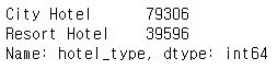
# 호텔 종류별 수 시각화

hotel["hotel_type"].value_counts().iplot(kind = "bar",
                                         layout = dict(
                                             title = dict(
                                                 text = "<b>호텔 종류별 수</b>",
                                                 font_size = 20),
                                             template = "plotly_white")
                                        )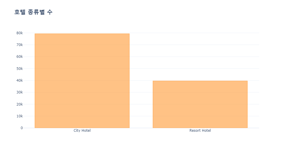
호텔은 City Hotel, Resort Hotel 두가지가 있으며 City Hotel 이 더 많이 있습니다.
# 전체 호텔 예약 취소 수

hotel["canceled"].value_counts()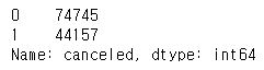
# 전체 호텔 예약 취소 비율

fig = px.pie(labels = hotel["canceled"].value_counts().index,
             values = hotel["canceled"].value_counts().values,
             names = ["No", "Yes"])


fig.update_traces(
    textinfo = "label + percent + value",
    textfont_size = 15,
    textfont_color = "white"
)

fig.update_layout(
    title = dict(
        text = "<b>전체 호텔 예약 취소 비율</b>",
        font_size = 20
    )
)

fig.show()
전체 예약 고객 중 약 37.1% 가 예약 취소를 합니다.
# 호텔별 예약 취소 비율

city_Hotel = hotel[hotel["hotel_type"] == "City Hotel"]
resort_Hotel = hotel[hotel["hotel_type"] == "Resort Hotel"]

fig = make_subplots(rows = 1, cols = 2, specs = [[{"type" : "pie"}, {"type" : "pie"}]])

fig.add_trace(
    go.Pie(labels = ["No", "Yes"],
           values = city_Hotel["canceled"].value_counts().values),
    row = 1, col = 1
)

fig.add_trace(
    go.Pie(labels = ["No", "Yes"],
           values = resort_Hotel["canceled"].value_counts().values),
    row = 1, col = 2
)

fig.update_traces(
    textinfo = "label + percent + value",
    textfont_size = 15,
    textfont_color = "white",
    hole = .4
)

fig.update_layout(
    title = dict(
        text = "<b>호텔 종류별 예약 취소 비율</b>",
        font_size = 20
    ),

    showlegend = False,

    # 파이 차트 가운데 글씨 넣기
    annotations = [dict(text = "City Hotel",
                        x = 0.175,
                        y = 0.505,
                        font_size = 15,
                        showarrow = False),
                   dict(text = "Resort Hotel",
                        x = 0.84,
                        y = 0.5,
                        font_size = 15,
                        showarrow = False)]
)

fig.show()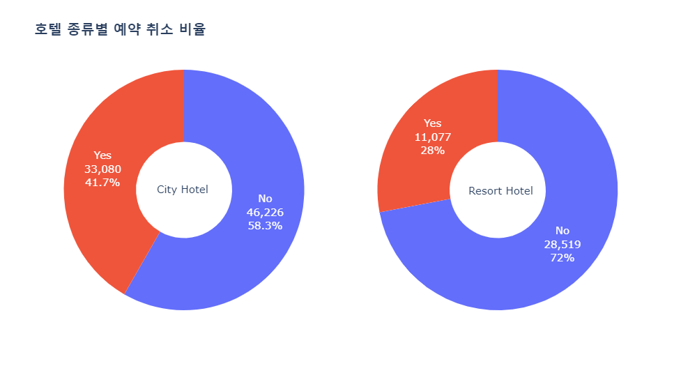
City Hotel 의 경우 전체 예약 고객 중 약 41.7% 가 취소를 하고, Resort Hotel 의 경우 전체 예약 고객 중 약 28% 가 취소를 합니다.
Resort Hotel 이 City Hotel 보다 예약 취소율이 더 낮습니다.
4-2 리드 타임과 예약 취소와의 관계는?
# 전체 예약 고객의 리드 타임 분포 시각화

hotel["lead_time"].iplot(kind = "box",
                         layout = dict(
                             title = dict(
                                 text = "<b>전체 예약 고객의 리드 타임 분포</b>",
                                 font_size = 20),
                             template = "plotly_white")
                        )
lead time 은 대부분 200일 안쪽으로 몰려 있습니다.
# 리드 타임과 예약 취소의 관계 시각화

fig = px.histogram(hotel[hotel["lead_time"] < 200], x = "lead_time", color = "canceled")

fig.update_layout(
    title = dict(
        text = "<b>리드 타임과 예약 취소의 관계</b>",
        font_size = 20
    ),

    legend = dict(
        title = "0:예약, 1:예약취소"
    ),

    template = "plotly_white"
)

fig.show()
리드 타임은 예약 취소 여부에 크게 영향을 미치지 않습니다.
4-3 언제 방문을 가장 많이 할까?
# 예약 취소를 하지 않은 고객 자료만 사용

hotel_booked = hotel[hotel["canceled"] == 0]

fig = make_subplots(rows = 3, cols = 1)

fig.add_trace(
    go.Bar(x = hotel_booked["arrival_date_year"].value_counts().index,
           y = hotel_booked["arrival_date_year"].value_counts().values,
           marker_color = color_1),
    row = 1, col = 1
)

fig.add_trace(
    go.Bar(x = hotel_booked["arrival_date_month"].value_counts().index,
           y = hotel_booked["arrival_date_month"].value_counts().values,
           marker_color = hotel_booked["arrival_date_month"].value_counts().values),
    row = 2, col = 1
)

fig.add_trace(
    go.Bar(x = hotel_booked["arrival_date_day_of_month"].value_counts().index,
           y = hotel_booked["arrival_date_day_of_month"].value_counts().values,
           marker_color = hotel_booked["arrival_date_day_of_month"].value_counts().values),
    row = 3, col = 1
)

fig.update_xaxes(title = "연도", dtick = 1, row = 1, col = 1)
fig.update_xaxes(title = "월", row = 2, col = 1)
fig.update_xaxes(title = "일", dtick = 1, row = 3, col = 1)

fig.update_layout(
    height = 1000,
    title = dict(
        text = "<b>연도별/월별/일별 호텔 방문 현황</b>",
        font_size = 20
    ),
    showlegend = False,
    template = "plotly_white"
)

fig.show()
2016년도에 가장 많이 호텔에 방문 했으며 주로 7,8월(여름)에 방문이 많습니다.
4-4 언제 예약 취소를 가장 많이 할까?
# 예약 취소한 고객 자료만 사용

hotel_canceled = hotel[hotel["canceled"] == 1]

fig = make_subplots(rows = 3, cols = 1)

fig.add_trace(
    go.Bar(x = hotel_canceled["arrival_date_year"].value_counts().index,
           y = hotel_canceled["arrival_date_year"].value_counts().values,
           marker_color = color_1),
    row = 1, col = 1
)

fig.add_trace(
    go.Bar(x = hotel_canceled["arrival_date_month"].value_counts().index,
           y = hotel_canceled["arrival_date_month"].value_counts().values,
           marker_color = hotel_canceled["arrival_date_month"].value_counts().values),
    row = 2, col = 1
)

fig.add_trace(
    go.Bar(x = hotel_canceled["arrival_date_day_of_month"].value_counts().index,
           y = hotel_canceled["arrival_date_day_of_month"].value_counts().values,
           marker_color = hotel_canceled["arrival_date_day_of_month"].value_counts().values),
    row = 3, col = 1
)

fig.update_xaxes(title = "연도", dtick = 1, row = 1, col = 1)
fig.update_xaxes(title = "월", row = 2, col = 1)
fig.update_xaxes(title = "일", dtick = 1, row = 3, col = 1)

fig.update_layout(
    height = 1000,
    title = dict(
        text = "<b>연도별/월별/일별 호텔 예약 취소 고객</b>",
        font_size = 20
    ),
    showlegend = False,
    template = "plotly_white"
)

fig.show()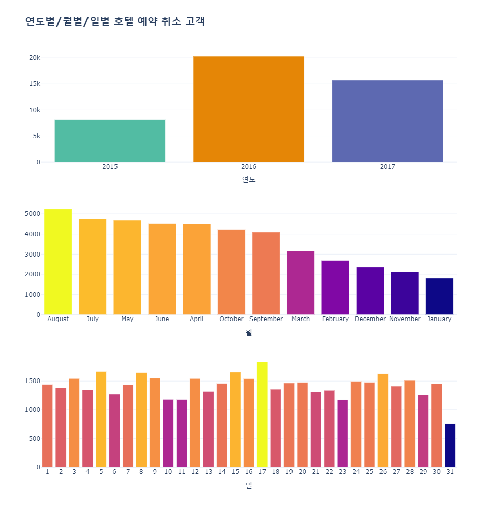
2016년에 가장 예약 취소가 많고 8월에 가장 예약 취소가 많습니다.
4-5 호텔에 얼마나 숙박을 할까?
# 주중, 주말 숙박일을 합쳐서 stays_in_total 컬럼에 등록

hotel_booked["stays_in_total"] = hotel_booked["stays_in_weekend_nights"] + hotel_booked["stays_in_week_nights"]

hotel_booked["stays_in_total"].head()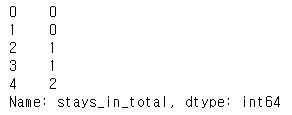
# 호텔 종류별 숙박일 시각화

hotel_stays = hotel_booked.groupby(["hotel_type","stays_in_total"]).agg({"lead_time" : "count"}).reset_index()
hotel_stays = hotel_stays.rename(columns = {"lead_time" : "count"})
hotel_stays = hotel_stays[hotel_stays["stays_in_total"] <= 31] # 1달이 최대 31일이므로, 31일 이내의 데이터만 추출

fig = px.bar(hotel_stays, x = "stays_in_total", y = "count",
             color = "hotel_type", barmode = "group")

fig.update_layout(
    title = dict(
        text = "<b>호텔 종류별 숙박일</b>",
        font_size = 20
    ),
    xaxis = dict(
        title = "총 숙박일",
        dtick = 1
    ),
    legend = dict(title = "호텔 종류"),
    template = "plotly_white"
)

fig.show()
City Hotel 의 경우 대부분 1일 ~ 4일 숙박을 하고, Resort Hotel 의 경우도 1일 ~ 4일 숙박하는 경우가 많지만 7일 숙박을 하는 경우가 두번째로 많은 것이 특징입니다.
4-6 호텔에 숙박하는 가족 수는 얼마나 될까?
# 성인, 아동/청소년, 유아 인원 수를 모두 더해 family 라는 컬럼에 등록

hotel_booked["family"] = hotel_booked["adults"] + hotel_booked["children"] + hotel_booked["babies"]

hotel_booked["family"].head()
# 호텔 종류별 가족 수 시각화

hotel_family = hotel_booked.groupby(["hotel_type","family"]).agg({"lead_time" : "count"}).reset_index()
hotel_family = hotel_family.rename(columns = {"lead_time" : "count"})

fig = px.bar(hotel_family, x = "family", y = "count",
             color = "hotel_type", barmode = "group")

fig.update_layout(
    title = dict(
        text = "<b>호텔 종류별 가족 수</b>",
        font_size = 20
    ),
    xaxis = dict(
        title = "가족 수",
        dtick = 1
    ),
    legend = dict(title = "호텔 종류"),
    template = "plotly_white"
)

fig.show()
두 호텔 다 2인 가족의 방문이 가장 많습니다.
4-7 호텔 식사 예약 비율은?
# 호텔 식사 종류별 예약 수

hotel["meal"].value_counts()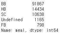
- Undefined/SC – no meal package
- BB – Bed & Breakfast
- HB – Half board (breakfast and one other meal – usually dinner)
- FB – Full board (breakfast, lunch and dinner)
# 호텔 식사 종류별 예약 비율 시각화

fig = px.pie(labels = hotel["meal"].value_counts().index,
             values = hotel["meal"].value_counts().values,
             names = hotel["meal"].value_counts().index)

fig.update_traces(
    textinfo = "label + percent",
    textposition = "auto",
    textfont_size = 15,
    textfont_color = "black"
)

fig.update_layout(
    title = dict(
        text = "<b>호텔 식사 종류별 예약 비율</b>",
        font_size = 20
    ),
    showlegend = False
)

fig.show()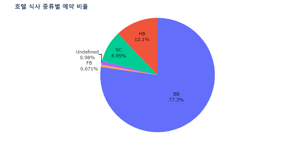
식사 예약은 대부분 BB 를 예약 합니다.
4-8 호텔에 가장 많이 방문하는 고객의 국가와 가장 많이 취소하는 고객의 국가는?
# 가장 많이 방문하는 고객의 국가 top10 데이터 추출

top10 = hotel_booked["country"].value_counts().nlargest(10).index
hotel_booked_top10 = hotel_booked[hotel_booked["country"].isin(top10)]

hotel_booked_top10["country"].unique()
# 가장 많이 방문하는 고객의 국가 top10 시각화

hotel_booked_country_top10 = hotel_booked_top10.groupby(["country", "hotel_type"]).agg({"canceled" : "count"}).reset_index()
hotel_booked_country_top10 = hotel_booked_country_top10.rename(columns = {"canceled" : "count"})

fig = px.bar(hotel_booked_country_top10, x = "country", y = "count", color = "hotel_type",
            barmode = "group")

fig.update_xaxes(
    categoryorder = "array",
    categoryarray = hotel_booked["country"].value_counts().index,
    title = "국가명"
)

fig.update_layout(
    title = dict(
        text = "<b>가장 많이 호텔에 방문하는 국가 Top10</b>",
        font_size = 20
    ),
    legend = dict(title = "호텔 종류"),
    template = "plotly_white"
)

fig.show()
포르투갈 국적의 고객이 모든 호텔에 가장 많이 방문합니다.
# 가장 많이 취소하는 고객의 국가 top10 데이터 추출

top10 = hotel_canceled["country"].value_counts().nlargest(10).index
hotel_canceled_top10 = hotel_canceled[hotel_canceled["country"].isin(top10)]

hotel_canceled_top10["country"].unique()
# 가장 많이 취소하는 고객의 국가 top10 시각화

hotel_canceled_country_top10 = hotel_canceled_top10.groupby(["country", "hotel_type"]).agg({"canceled" : "count"}).reset_index()
hotel_canceled_country_top10 = hotel_canceled_country_top10.rename(columns = {"canceled" : "count"})

fig = px.bar(hotel_canceled_country_top10, x = "country", y = "count", color = "hotel_type",
            barmode = "group")

fig.update_xaxes(
    categoryorder = "array",
    categoryarray = hotel_canceled["country"].value_counts().index,
    title = "국가명"
)

fig.update_layout(
    title = dict(
        text = "<b>가장 많이 예약 취소하는 국가 Top10</b>",
        font_size = 20
    ),
    legend = dict(title = "호텔 종류"),
    template = "plotly_white"
)

fig.show()
가장 많이 취소하는 국가도 포르투갈이며, City Hotel 취소 비율이 Resort Hotel 보다 훨씬 높은 것이 특징입니다.
'Data Analysis > Kaggle' 카테고리의 다른 글
| [Kaggle] Hotel Booking Demand 데이터셋 분석 2 (데이터 전처리) (0) | 2021.11.08 |
|---|---|
| [Kaggle] Hotel Booking Demand 데이터셋 분석 1 (데이터 확인 / 질문) (0) | 2021.11.08 |
| [Kaggle] Students Performance in Exam 데이터 분석 2 (EDA / 시각화 / 리뷰) (0) | 2021.11.05 |
| [Kaggle] Students Performance in Exam 데이터 분석 1 (데이터 확인 / 질문 / 전처리) (0) | 2021.11.03 |
| [Kaggle] Nexfilx movies and TV shows 데이터 분석 3 (EDA / 시각화 / Review) (0) | 2021.11.02 |


